Predicting Rainfall and Flooding With a CNN-LSTM Hybrid

The Problem

Flooding is one of the most destructive and hard-to-predict natural events. The challenge is not just about knowing how much rain will fall. It is about understanding how water moves through a landscape over time. Rainfall at one point affects conditions downstream minutes or hours later. Static snapshots miss this entirely.

And critically, flooding is not a binary event. An area is not simply flooded or not flooded. Severity exists on a spectrum, from surface water accumulation to complete inundation. Any model worth building needs to reflect that: predicting a continuous severity field across the full spatial grid, not a yes or no label.

What you actually need is a model that understands both space and time simultaneously. A model that can look at a sequence of rainfall or flood frames and say: given what I have seen so far, here is what comes next.

That is what this project set out to build.

The Architecture

The core intuition is straightforward. CNNs are excellent at extracting spatial features from a frame: patterns, textures, structures. LSTMs are excellent at learning sequences over time. Combining them gives a model that can extract spatial features from each frame and then reason about how those features evolve across a sequence.

The architecture I built (conv_lstm) chains two convolutional stages into two stacked LSTM layers, followed by fully connected layers that project down to the output prediction.

Convolutional Stage

Two Conv2D layers extract spatial features from each input frame:

• Layer 1: 1 input channel to 10 feature maps, 3x3 kernel, followed by BatchNorm2D, ReLU, and average pooling with a (2,4) kernel
• Layer 2: 10 to 10 feature maps, 2x2 kernel, followed by BatchNorm2D, ReLU, and average pooling with a (2,2) kernel

Weights are initialised using the inverse square root of the fan-in. That keeps activations stable from the first forward pass rather than relying on random initialisation to sort itself out during early training.

The choice of average pooling over max pooling was deliberate for this domain. Max pooling picks the strongest activation and discards everything else. For rainfall data, where gradual spatial gradients matter more than sharp peaks, average pooling preserves the distributed signal more faithfully.

LSTM Stage

After the convolutional layers flatten and compress the spatial features, two stacked LSTM layers with hidden size 512 process the temporal sequence:

• LSTM layer 1: takes the conv output directly, 2 layers, 20% dropout
• LSTM layer 2: takes the output of LSTM 1, 2 layers, 5% dropout

Stacking allows the first LSTM to learn lower-level temporal patterns and the second to reason about higher-level dynamics. Hidden and cell states are initialised to zero at the start of each sequence.

Fully Connected Output

The final hidden state from the second LSTM is taken at the last timestep only, flattened, and passed through:

• FC layer: 2560 to 2560
• LayerNorm
• ReLU
• FC layer: 2560 to 100 (the output prediction)

LayerNorm on the bottleneck was added to stabilise training. Without it, the large fully connected layers produced unstable gradient flow during early epochs.

The Data Pipeline

Input data is organised as sequential frames. Each sample is a frame at time T, and the label is the corresponding frame at time T+1. The model learns to predict the next state of the system given the current one.

The custom dataloader (conv_lstm_dataloader) reads frame tensors from disk, pairs them with their output tensors, and feeds them into the training loop. The dataset is split 69 training samples to 9 test samples, with a batch size of 1. That is appropriate given the sequential nature of the data, where shuffling the test set would break temporal coherence.

Training uses MSE loss and the Adam optimiser at a learning rate of 0.0001. MSE is the natural choice here since the output is a continuous spatial field rather than a discrete class.

Two Prediction Modes

One of the more interesting design decisions was implementing two distinct test modes.

Standard mode (test_model): the model receives the true frame at each timestep and predicts the next one. It always has access to ground truth as its input.

Force-feed mode (test_model_force_feed_out): the model is given only the first real frame. After that, its own prediction becomes the input for the next step. The model is essentially generating a sequence from a single seed frame, with each prediction feeding directly into the next.

Understanding the Visualisation

Before looking at the results, it helps to understand what the pixel values actually represent.

Each frame is a greyscale spatial grid where pixel intensity encodes flood severity on a 0 to 255 scale:

• Black (0): no flooding
• Mid grey (~128): moderate flooding, roughly halfway to worst case
• White (255): maximum flood severity

So a frame that is mostly black with a few bright patches is showing isolated severe flooding against a dry background. A frame that is uniformly mid-grey represents widespread moderate flooding across the entire area. The model is not predicting a binary flooded or not flooded label. It is predicting a continuous severity field across the full spatial grid.

Predictions vs Ground Truth

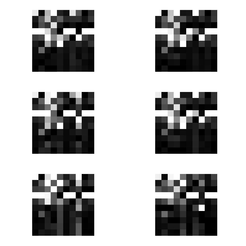
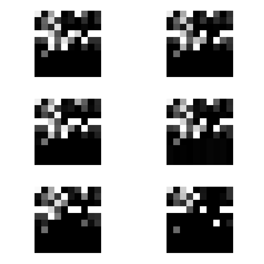
The GIFs below show the model's force-feed predictions alongside the ground truth sequence. The upper spatial structure tracks closely across multiple steps. The lower region shows gradual drift accumulating over time, which is the expected behaviour when the model is generating purely from its own outputs rather than receiving real input.

What the Results Showed

The model produces spatially coherent frame predictions that track the broad structure of the true sequence. The force-feed mode holds together across multiple steps before gradual drift accumulates, which confirms the model has learned real temporal dynamics rather than just memorising inputs.

The loss curve (saved as avg-pooling-10-channel.png) shows consistent descent across the 10 training epochs, with no signs of instability from the LayerNorm and BatchNorm combination.

What I Would Do Differently Now

This was a prototype. Looking back at it with more experience, a few things stand out.

The architecture predates ConvLSTM cells. The paper referenced in the repo (Shi et al., 2015) proposes doing the convolution inside the LSTM cell rather than feeding conv outputs into a separate LSTM. That approach maintains spatial structure through the temporal processing rather than collapsing it first. My implementation does the convolution and LSTM sequentially, which is a reasonable first approach but not the same thing as a true ConvLSTM cell.

The dataset is small. 78 samples total is a prototype constraint. Real spatiotemporal flood prediction would need significantly more data to generalise across different rainfall patterns and terrain types.

Attention would help. Adding a spatial attention mechanism between the CNN and LSTM would let the model learn which spatial regions matter most for predicting the next timestep, rather than treating all spatial features equally.

Why This Problem Matters

Flood prediction is not just an academic exercise. Early warning systems that can predict where water will move and when can save lives. The ability to generate multi-step predictions from a single seed frame is exactly what makes this approach potentially useful in practice. You do not need continuous sensor input to run the model forward; you need a starting state and a model that has learned the physics well enough to extrapolate.

This project was a prototype. But the architecture direction is sound, and the problem is one worth continuing to work on.

Attribution

The ConvLSTM architecture explored in this project is based on published academic research. The original paper is:

Shi, X., Chen, Z., Wang, H., Yeung, D. Y., Wong, W. K., & Woo, W. C. (2015). Convolutional LSTM Network: A Machine Learning Approach for Precipitation Nowcasting. arXiv:1506.04214. arxiv.org/abs/1506.04214

This implementation is an independent re-implementation of the concepts described in the paper, built from scratch in PyTorch for learning and research purposes.

Full source: github.com/Kikumu/Flood-algo-draft